By Abhay bansal — Nov 26, 2020

THE MATHS BEHIND LOGISTIC REGRESSION

WHAT IS LOGISTIC REGRESSION?

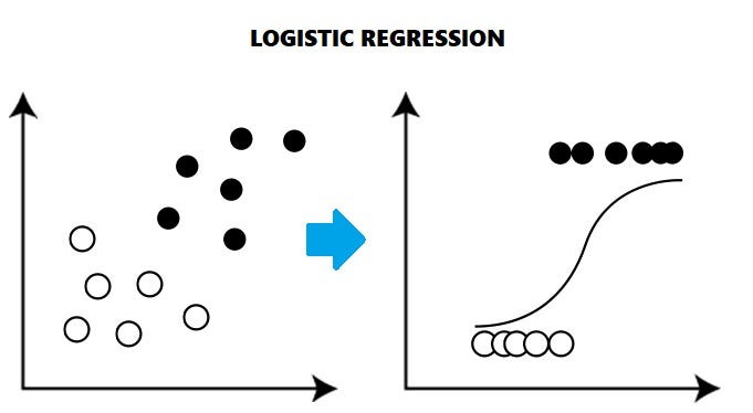
Logistic Regression is a Supervised statistical technique to find the probability of dependent variable(Classes present in the variable).

SIGMOID FUNCTION

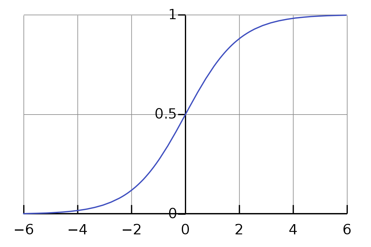
In order to map predicted values to probabilities, we use the sigmoid function. The function maps any real value into another value between 0 and 1. In machine learning, we use sigmoid to map predictions to probabilities.

def sigmoid(z): return 1.0 / (1 + np.exp(-z))

LOGISTIC REGRESSION PROCESS

Given a data(X,Y), X being a matrix of values with m examples and n features and Y being a vector with m examples. The objective is to train the model to predict which class the future values belong to. Primarily, we create a weight matrix with random initialisation. Then we multiply it by features.

We then pass the above equation into the sigmoid function defined earlier.

def predict(features, weights): //Returns 1D array of probabilities that the class label == 1 z = np.dot(features, weights) return sigmoid(z)

COST FUNCTION

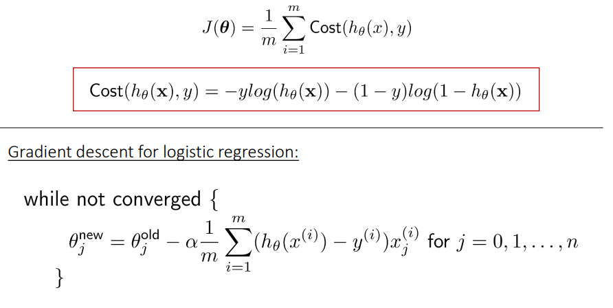
Instead of Mean Squared Error, we use a cost function called Cross-Entropy, also known as Log Loss. Cross-entropy loss can be divided into two separate cost functions: one for y=1 and one for y=0.

The benefits of taking the logarithm reveal themselves when you look at the cost function graphs for y=1 and y=0. These smooth monotonic functions [7] (always increasing or always decreasing) make it easy to calculate the gradient and minimise cost. Image from Andrew Ng’s slides on logistic regression [1].

def cost_function(features, labels, weights):
    '''
    Using Mean Absolute Error
    Features:(100,3)
    Labels: (100,1)
    Weights:(3,1)
    Returns 1D matrix of predictions
    Cost = (labels*log(predictions) + (1-labels)*log(1-predictions) ) / len(labels)
    '''
    observations = len(labels)

    predictions = predict(features, weights)

    #Take the error when label=1
    class1_cost = -labels*np.log(predictions)

    #Take the error when label=0
    class2_cost = (1-labels)*np.log(1-predictions)

    #Take the sum of both costs
    cost = class1_cost - class2_cost

    #Take the average cost
    cost = cost.sum() / observations

    return cost

GRADIENT DESCENT

To minimise our cost, we use Gradient Descent just like before in Linear Regression. There are other more sophisticated optimisation algorithms out there such as conjugate gradient like BFGS, but you don’t have to worry about these. Machine learning libraries like Scikit-learn hide their implementations so you can focus on more interesting things!

s′(z)=s(z)(1−s(z))

`def update_weights(features, labels, weights, lr):
'''
Vectorized Gradient Descent

Features:(200, 3)
Labels: (200, 1)
Weights:(3, 1)
'''
N = len(features)

#1 - Get Predictions
predictions = predict(features, weights)

#2 Transpose features from (200, 3) to (3, 200)
# So we can multiply w the (200,1)  cost matrix.
# Returns a (3,1) matrix holding 3 partial derivatives --
# one for each feature -- representing the aggregate
# slope of the cost function across all observations
gradient = np.dot(features.T,  predictions - labels)

#3 Take the average cost derivative for each feature
gradient /= N

#4 - Multiply the gradient by our learning rate
gradient *= lr

#5 - Subtract from our weights to minimize cost
weights -= gradient

return weights`

REFERENCES

How is the cost function from Logistic Regression derivated

I am doing the Machine Learning Stanford course on Coursera. In the chapter on Logistic Regression, the cost function is this: Then, it is derivated here: I tried getting the derivative of the c...

Cross Validatedoctavian

https://ml-cheatsheet.readthedocs.io/en/latest/logistic_regression.html