Linear Regression (Scary Math + Doable Practicality)

Just like how you still remember and think about the days when you and your first crush were together, every MLE and DS who has studied the scary Math behind Transformers and other advanced models remembers those old days when they had to deal with Linear Regression.

Linear Regression seldom is not the starting point for pretty much every guy who deals with Data and ML models. So, let's take a deep dive in this Blog as to what is Linear Regression. I will covering the parts of understading Linear Regression through underlying Math and then writing it from scratch and trying it out on a Dataset.

So, what is Linear Regression? If you remember correctly, Linear Regression falls under the category of Supervised Learning which just means training a model by providing it with some help (a dataset) in this case. Linear Regression at it's very core is just Curve - Fitting which means we need to find a curve which perfectly fits some given co - ordinates on a given co - ordinate system. That curve can be a simple straight line y = mx + c (or y = mx + b) to some higher Polynomial (Quadratic, Cubic, etc).

Linear Regression, as the name suggests is Linear, i.e., is represented by y = mx + c where m is the slope of the line and c being the y - intercept. (This equation can vary on the basis of the number of features our Problem Statement is dealing with. For ex, a Dataset with 2 features will make the equation as y = m1 * x1 + m2 * x2 + c, etc).

So, this is a little introduction to Linear Regression and it's ~(difficult) representation.

Let's go a bit deeper

In reality, we do not use the notations we are using here. The picture below shows the exact same equation we saw above but using the main notations.

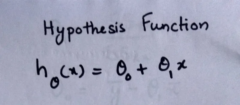
Here, h(x) to the subscript theta represents the Hypothesis Function. It's nothing to be scared of. This line just says that Assuming that the relationship between my input feature and the output feature is linear, what are the best values of Theta 0 and Theta 1 that we can get.

So, this is how we prefer representing Linear Regression.

Now that we know what equation we use represent our Linear Regression model, let's see some more things related to it.

Now, it's important to understand this line will represent a specific straight line which may or may not be the best line to fit the data. Let's understand this with the help of the image below

Let's say for the data points (Black colour), we get the following fit line (Green colour). Now, we can clearly tell that this line is not able to fit the data points accurately and so, we need to update the value of Theta 0 and Theta 1 (m and c respectively) and for that, we use a process known as Gradient Descent. This algorithm also lays the foundation for Neural Networks and a process in it known as Backpropagation.

So, now let's understand what is Gradient Descent, how do we represent it in Math and how does it end up giving us the best values for Theta 0 and Theta 1.

Gradient Descent is a process with the help of which we can update the values of Theta 1 and Theta 0 which eventually gives us the best line which can fit our data.

We can understand it with the help of the following image shown below,

So, this is the image of Loss function, which tells us the total amount of mistakes that we've performed during evaluating with our current curve (straight line in this case). The representation of this Loss Function is shown below. Again, h(x) to the subscript i represents the current prediction that we've made and we subtract the Expected Output (Actual Answer). Now this is the same Mean Squared Error function that we use quite oftenly in Regression tasks but the 1 / 2 might be a bit confusing here. So, when we take the derivative of this function (which we'll do in a bit), we get a 2 in the numerator which gets cancelled out by the 2 in the denominator. It's just for some cleaniness and simplicity and holds no other significance.

So, now that we know which Cost function we are going to use, we can go back to the inverted Bell Curve above. So, this cost function is represented by the Inverted Bell curve above and we need to get as near to the Minimum position as possible and that's what Gradient Descent is. Going from top the Curve to the very minimum value. This Minimum value is also known as the Minima and it can be either Global Minima or Local Minima (Its always preferable to reach the Global Minima).

Now let's understand how math helps us reach the minimum possible position by taking some derivatives. Again, in the whole process, Theta 0 represents the y - intercept and Theta 1 represents the slope m.

In the image above, we are taking the partial derivative of the Cost function with respect to Theta 0 first and then Theta 1 and finally, updating them with their new values. For this, we also use the Learning Rate (LR).

Now, let's spend a minute on Learning Rate. While we are trying to move from the top to the minimum value of the Inverted bell curve, Learning Rate controls at what speed are we trying to come to the Minima of the Cost Function. It's always preferred for the LR to be around quite low (in terms 0.001 or lower or just a bit higher). The perfect Learning Rate can only be found by experimenting. But abstain from keeping the Learning Rate too high or too low as it can lead to discrepancies.

We do this Gradient Descent Process for many many times (Epochs) and end with the final value that we will be using for our best fit line.

Too much talking, right? Let's code

I will be using Google Colab for this. You can choose any IDE of your liking.

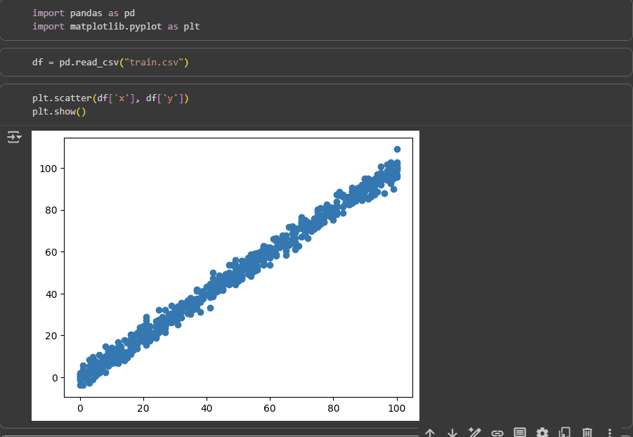
I initially make the few required imports and check the train.csv that I have.

This dataset has been taken deliberately in such a way that we can implement whatever we have learnt today

Now the above code is how we define our Cost Function (or Loss Function). data represents the Dataframe that we are going to be using. We iterate over the total number of samples (rows) of data that we have and calculate the difference between the Predicted values and the actual values. Note: Here, the formula we've written here might seem different from the one we had written above but it doesn't make a difference because we are taking the square in the end, so, it's the exact same value.

Although writing the Loss Function isn't preferable as we should write the Loss Function and the Gradient Descent together. So, you can just understand the above function for reference.

Let's write the Gradient Descent Function -

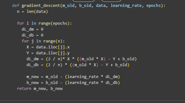
Here, we have the written the Gradient Descent function as we had defined it earlier. In this function, we define the number of epochs that we want to take to update and find the best value for m and b which we are calling m_new and b_new here. Numbers of Epochs can vary and they too need a lot of experimentation to find the best estimate.

Now, we just give the values for all the parameters required in the Gradient Descent Function. Note: the initial values of m, b and the value of LR are always experimented to find the best fit

Finally, we define the x_min and x_max values to plot the Regression Line with the Scattered data.

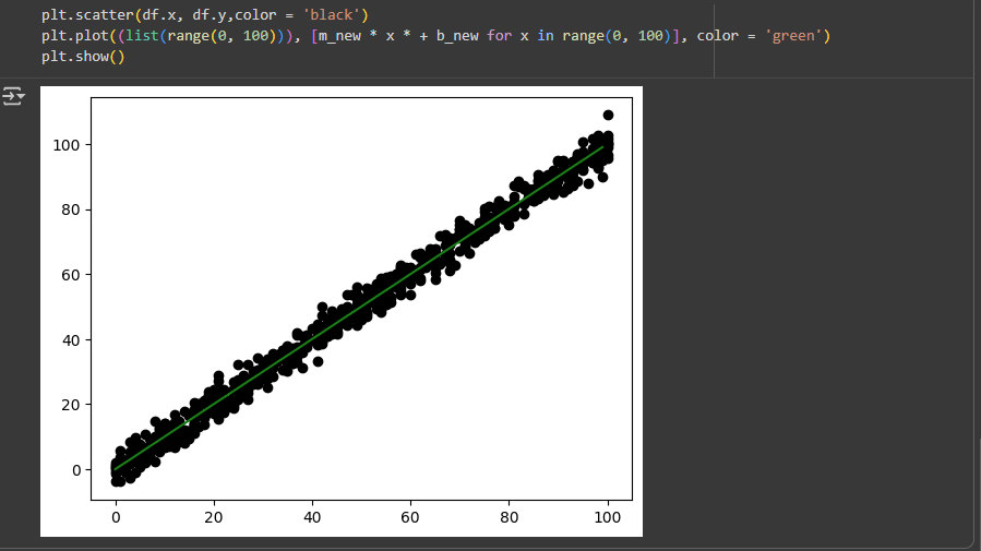
So, as we can see, we have successfully found the best fit line for this dataset. This did take me a lot of time by experimenting with different values of the parameters of Gradient Descent so playing around and experimenting with different hyper - parameters (known as Hyper - parameter tuning) is a crucial part of a MLE or DS's life.

So, this brings us to the end of this Blog. Hope I was able to impart knowledge to you guys. You can watch multiple videos on building Linear Regression from scratch to better understand this concept if you were not able to understand this blog properly.

In the upcoming blogs, we'll cover more such Models and build them from scratch.